Chapter 1 Getting started

XSHELLS is yet another code simulating incompressible fluids in a spherical cavity. In addition to the Navier-Stokes equation with an optional Coriolis force, it can also time-step the coupled induction equation for MHD (with imposed magnetic field or in a dynamo regime), as well as the temperature (and concentration) equation in the Boussinesq framework.

XSHELLS uses finite differences (second order) in the radial direction and spherical harmonic decomposition (pseudo-spectral). The time-stepping uses a highly stable, second order, semi-implicit, predictor-corrector scheme (with only diffusive terms treated implicitly).

XSHELLS is written in C++ and designed for speed. It uses the blazingly fast spherical harmonic transform library SHTns, as well as hybrid parallelization using OpenMP and/or MPI. This allows it to run efficiently on your laptop or on parallel supercomputers. A post-processing program is provided to extract useful data and export fields to python/matplotlib or paraview.

XSHELLS is free software, distributed under the CeCILL Licence (compatible with GNU GPL): everybody is free to use, modify and contribute to the code.

Grab the XSHELLS archive and extract it. Alternativley, you can use git to clone the repository

git clone --recurse-submodules https://bitbucket.org/nschaeff/xshells.git

If you need to install XSHELLS manually (e.g. because the above easy installation fails or you need a specific configuration not covered by the wizard), here are some useful details.

There are two configuration files:

• •

  xshells.hpp is read by the compiler (compile-time options), and modifying it requires to recompile the program. The corresponding options are detailed in section 2.2.

• •

  xshells.par is read by the program at startup (runtime options) and modifying it does not require to recompile the program. This file is detailed in section 2.1.

See chapter 2 for more details. Example configuration files can be found in the problems directory.

Before compiling, copy the configuration files that correspond most closely to your problem. For example, the geodynamo benchmark:

  cp problems/geodynamo/xshells.par .
  cp problems/geodynamo/xshells.hpp .

and then edit them to adjust the parameters (see sections 2.2 and 2.1).

When you have properly set the xshells.hpp and xshells.par files, you can compile and run in different flavours:

All output files are suffixed by the job name as file extension, denoted job in the following. The various output files are:

• •

  xshells.par.job : a copy of the input parameter file xshells.par, for future reference.

• •

  xshells.hpp.job : a stripped-out version of the file xshells.hpp that was used during compilation, for future reference.

• •

  energy.job : a record of energies and other custom diagnostics. Each line of this text file is an iteration.

• •

  fieldX0.job : the imposed (constant) field X, if any.

• •

  fieldX_####.job : the field X at iteration number ####, if parameter movie was set to a non-zero value in xshells.par.

• •

  fieldXavg_####.job : the field X averaged between previous iteration and iteration number ####, if parameter movie was set to 2 in xshells.par.

• •

  fieldX.job : the last full backup of field X, or field X at the end of the simulation. Used when restarting a job.

All field files are binary format files storing the spherical harmonic coefficients of the field. To produce plots and visualizations, they can be post-processed using the xspp program (see chapter 3).

The parallelization of XSHELLS is done by domain decomposition in the radial direction only, using MPI. In addition to this domain decomposition, shared memory parallelism is implemented using OpenMP. Furthermore, MPI-3 shared memory can be used for communications between processes on the same node, with significant performance gains, and somehow mimicking a two-dimensional domain decomposition. The MPI-3 shared memory solver in XSHELLS requires a cache-coherent architecture, and is currently enabled by default only on x86 machines. To enable or tune MPI-3 shared memory, add -shared_mem=N to the command line, with N the number of cores that should share memory.

There are four variants of the code that differ in the way OpenMP is used:

• •

  xsbig uses only OpenMP in the radial direction (no MPI). It can only run on a single node, but does not need an MPI library. This is good for a general purpose desktop or laptop computer, but also on NUMA nodes (although some MPI may lead to better performance). Low memory usage.

• •

  xsbig_mpi uses only MPI in the radial direction (no OpenMP). This is good for medium sized problems, running on small clusters.

• •

  xsbig_hyb uses both MPI and OpenMP in the radial direction, to reduce the number of MPI processes and memory usage. As a consequence, it is more efficient to use a number of radial shells that is a multiple of the number of computing cores. Beyond 1 thread per radial shell (or in case of imbalance), OpenMP tasks are used to share the work of one shell across several threads, although this leads to a less than ideal scaling.

• •

  xsbig_hyb2 uses MPI in the radial direction and OpenMP within a radial shell. This strategy usually performs well, allows to efficiently address more computing cores, but uses a lot of memory (an order of magnitude more than xsbig_hyb). It is highly recommended to use a number of radial shells that is a multiple of the number of nodes. This mode cannot go beyond 1 MPI process per radial shell, but intra-node shared memory parallelism allows to use all cores of a single node within each process. Note also that the SHTns library compiled with OpenMP is needed.

In any case, the number of MPI processes cannot exceed the total number of radial shells. It is often more efficient to use a small number of MPI processes per node (1 to 4) and use OpenMP to have a total number of threads equal to the number of cores.

Because there is no automatic load balancing, some situations where the same amount of work is not required for each radial shell will result in suboptimal scaling when the number of MPI processes is increased. Such situations include (i) solid conducting shells (e.g. a conducting inner core) and (ii) variable spherical harmonic degree truncation (e.g. in a full-sphere problem). In these cases, especially the latter, use pure OpenMP or minimize the number of MPI processes.

Using MPI executables (including hybrid MPI+OpenMP) is thus optimal only if the following conditions are both met:

• •

  all fields span the same radial domain (no conducting solid shells);

• •

  the radial domain does not include the center $r=0$ (and XS_VAR_LTR is not used, see section 2.2.4).

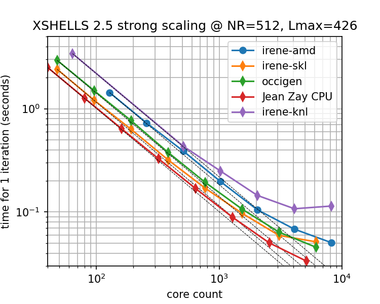
In such cases, XSHELLS should scale very well up to the limit of 1 thread per radial shell, and even beyond with the in-shell OpenMP mode of xsbig_hyb2 (see scaling example in Figure 1.1).

If you use XSHELLS for research work, you should cite the SHTns paper (because the high performance of XSHELLS is mostly due to the blazingly fast spherical harmonic transform provided by SHTns):

N. Schaeffer, Efficient Spherical Harmonic Transforms aimed at pseudo-spectral numerical simulations, Geochem. Geophys. Geosyst. 14, 751-758, doi:10.1002/ggge.20071 (2013)

In addition, depending on the problem you solve, you could cite:

• •

  Geodynamo:
  N. Schaeffer et. al, Turbulent geodynamo simulations: a leap towards Earth’s core, Geophys. J. Int. doi:10.1093/gji/ggx265 (2017)

• •

  Spherical Couette:
  A. Figueroa et. al, Modes and instabilities in magnetized spherical Couette flow, J. Fluid Mech. doi:10.1017/jfm.2012.551 (2013)

• •

  Full-spheres: E. Kaplan et. al, Subcritical thermal convection of liquid metals in a rapidly rotating sphere, Phys. Res. Lett. doi:10.1103/PhysRevLett.119.094501 (2017)

• •

  Kinematic dynamos:
  N. Schaeffer et. al, Can Core Flows inferred from Geomagnetic Field Models explain the Earth’s Dynamo ?, Geophys. J. Int. doi:10.1093/gji/ggv488 (2016)