shallow_water.py
Solves the non-linear barotropically unstable shallow water test case in Python.
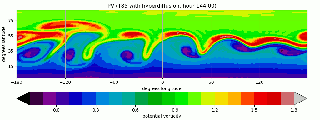
Solves the non-linear barotropically unstable shallow water test case in Python. Running the script should pop up a window with this image:
1#! /usr/bin/env python3
2
3#
4# "Non-linear barotropically unstable shallow water test case"
5# Example provided by Jeffrey Whitaker
6# https://gist.github.com/jswhit/3845307
7#
8# Running the script should pop up a window with this image:
9# https://i.imgur.com/CEzHJ0g.png
10#
11
12import numpy as np
13import shtns
14
15
16class Spharmt(object):
17 """
18 wrapper class for commonly used spectral transform operations in
19 atmospheric models. Provides an interface to shtns compatible
20 with pyspharm (pyspharm.googlecode.com).
21 """
22 def __init__(self, nlons, nlats, ntrunc, rsphere, gridtype="gaussian"):
23 """initialize
24 nlons: number of longitudes
25 nlats: number of latitudes"""
26 self._shtns = shtns.sht(ntrunc, ntrunc, 1,
27 shtns.sht_orthonormal+shtns.SHT_NO_CS_PHASE)
28
29 if gridtype == "gaussian":
30 # self._shtns.set_grid(nlats, nlons,
31 # shtns.sht_gauss_fly | shtns.SHT_PHI_CONTIGUOUS, 1.e-10)
32 self._shtns.set_grid(nlats, nlons,
33 shtns.sht_quick_init | shtns.SHT_PHI_CONTIGUOUS, 1.e-10)
34 elif gridtype == "regular":
35 self._shtns.set_grid(nlats, nlons,
36 shtns.sht_reg_dct | shtns.SHT_PHI_CONTIGUOUS, 1.e-10)
37
38 self.lats = np.arcsin(self._shtns.cos_theta)
39 self.lons = (2.*np.pi/nlons)*np.arange(nlons)
40 self.nlons = nlons
41 self.nlats = nlats
42 self.ntrunc = ntrunc
43 self.nlm = self._shtns.nlm
44 self.degree = self._shtns.l
45 self.lap = -self.degree*(self.degree+1.0).astype(complex)
46 self.invlap = np.zeros(self.lap.shape, self.lap.dtype)
47 self.invlap[1:] = 1./self.lap[1:]
48 self.rsphere = rsphere
49 self.lap = self.lap/rsphere**2
50 self.invlap = self.invlap*rsphere**2
51
52 def grdtospec(self, data):
53 """compute spectral coefficients from gridded data"""
54 return self._shtns.analys(data)
55
56 def spectogrd(self, dataspec):
57 """compute gridded data from spectral coefficients"""
58 return self._shtns.synth(dataspec)
59
60 def getuv(self, vrtspec, divspec):
61 """compute wind vector from spectral coeffs of vorticity and divergence"""
62 return self._shtns.synth((self.invlap/self.rsphere)*vrtspec, (self.invlap/self.rsphere)*divspec)
63
64 def getvrtdivspec(self, u, v):
65 """compute spectral coeffs of vorticity and divergence from wind vector"""
66 vrtspec, divspec = self._shtns.analys(u, v)
67 return self.lap*self.rsphere*vrtspec, self.lap*rsphere*divspec
68
69 def getgrad(self, divspec):
70 """compute gradient vector from spectral coeffs"""
71 vrtspec = np.zeros(divspec.shape, dtype=complex)
72 u, v = self._shtns.synth(vrtspec, divspec)
73 return u/rsphere, v/rsphere
74
75
76if __name__ == "__main__":
77 import matplotlib.pyplot as plt
78 import time
79
80 # non-linear barotropically unstable shallow water test case
81 # of Galewsky et al (2004, Tellus, 56A, 429-440).
82 # "An initial-value problem for testing numerical models of the global
83 # shallow-water equations" DOI: 10.1111/j.1600-0870.2004.00071.x
84 # http://www-vortex.mcs.st-and.ac.uk/~rks/reprints/galewsky_etal_tellus_2004.pdf
85
86 # requires matplotlib for plotting.
87
88 # grid, time step info
89 nlons = 256 # number of longitudes
90 ntrunc = int(nlons/3) # spectral truncation (for alias-free computations)
91 nlats = int(nlons/2) # for gaussian grid.
92 dt = 150 # time step in seconds
93 itmax = 6*int(86400/dt) # integration length in days
94
95 # parameters for test
96 rsphere = 6.37122e6 # earth radius
97 omega = 7.292e-5 # rotation rate
98 grav = 9.80616 # gravity
99 hbar = 10.e3 # resting depth
100 umax = 80. # jet speed
101 phi0 = np.pi/7.
102 phi1 = 0.5*np.pi - phi0
103 phi2 = 0.25*np.pi
104 en = np.exp(-4.0/(phi1-phi0)**2)
105 alpha = 1./3.
106 beta = 1./15.
107 hamp = 120. # amplitude of height perturbation to zonal jet
108 efold = 3.*3600. # efolding timescale at ntrunc for hyperdiffusion
109 ndiss = 8 # order for hyperdiffusion
110
111 # setup up spherical harmonic instance, set lats/lons of grid
112 x = Spharmt(nlons, nlats, ntrunc, rsphere, gridtype="gaussian")
113 lons, lats = np.meshgrid(x.lons, x.lats)
114 f = 2.*omega*np.sin(lats) # coriolis
115
116 # zonal jet.
117 vg = np.zeros((nlats, nlons), float)
118 u1 = (umax/en)*np.exp(1./((x.lats-phi0)*(x.lats-phi1)))
119 ug = np.zeros((nlats), float)
120 ug = np.where(np.logical_and(x.lats < phi1, x.lats > phi0), u1, ug)
121 ug.shape = (nlats, 1)
122 ug = ug*np.ones((nlats, nlons), dtype=float) # broadcast to shape (nlats, nlonss)
123 # height perturbation.
124 hbump = hamp*np.cos(lats)*np.exp(-((lons-np.pi)/alpha)**2)*np.exp(-(phi2-lats)**2/beta)
125
126 # initial vorticity, divergence in spectral space
127 vrtspec, divspec = x.getvrtdivspec(ug, vg)
128 vrtg = x.spectogrd(vrtspec)
129 divg = x.spectogrd(divspec)
130
131 # create hyperdiffusion factor
132 hyperdiff_fact = np.exp((-dt/efold)*(x.lap/x.lap[-1])**(ndiss/2))
133
134 # solve nonlinear balance eqn to get initial zonal geopotential,
135 # add localized bump (not balanced).
136 vrtg = x.spectogrd(vrtspec)
137 tmpg1 = ug*(vrtg+f)
138 tmpg2 = vg*(vrtg+f)
139 tmpspec1, tmpspec2 = x.getvrtdivspec(tmpg1, tmpg2)
140 tmpspec2 = x.grdtospec(0.5*(ug**2+vg**2))
141 phispec = x.invlap*tmpspec1 - tmpspec2
142 phig = grav*(hbar + hbump) + x.spectogrd(phispec)
143 phispec = x.grdtospec(phig)
144
145 # initialize spectral tendency arrays
146 ddivdtspec = np.zeros(vrtspec.shape+(3,), complex)
147 dvrtdtspec = np.zeros(vrtspec.shape+(3,), complex)
148 dphidtspec = np.zeros(vrtspec.shape+(3,), complex)
149 nnew = 0
150 nnow = 1
151 nold = 2
152
153 # time loop.
154 time1 = time.time()
155 for ncycle in range(itmax+1):
156 t = ncycle*dt
157 # get vort, u, v, phi on grid
158 vrtg = x.spectogrd(vrtspec)
159 ug, vg = x.getuv(vrtspec, divspec)
160 phig = x.spectogrd(phispec)
161 print("t=%6.2f hours: min/max %6.2f, %6.2f" % (t/3600., vg.min(), vg.max()))
162
163 # compute tendencies.
164 tmpg1 = ug*(vrtg+f)
165 tmpg2 = vg*(vrtg+f)
166 ddivdtspec[:, nnew], dvrtdtspec[:, nnew] = x.getvrtdivspec(tmpg1, tmpg2)
167 dvrtdtspec[:, nnew] *= -1
168
169 tmpg = x.spectogrd(ddivdtspec[:, nnew])
170 tmpg1 = ug*phig
171 tmpg2 = vg*phig
172 tmpspec, dphidtspec[:, nnew] = x.getvrtdivspec(tmpg1, tmpg2)
173 dphidtspec[:, nnew] *= -1
174
175 tmpspec = x.grdtospec(phig+0.5*(ug**2+vg**2))
176 ddivdtspec[:, nnew] += -x.lap*tmpspec
177
178 # update vort, div, phiv with third-order adams-bashforth.
179 # forward euler, then 2nd-order adams-bashforth time steps to start.
180 if ncycle == 0:
181 dvrtdtspec[:, nnow] = dvrtdtspec[:, nnew]
182 dvrtdtspec[:, nold] = dvrtdtspec[:, nnew]
183 ddivdtspec[:, nnow] = ddivdtspec[:, nnew]
184 ddivdtspec[:, nold] = ddivdtspec[:, nnew]
185 dphidtspec[:, nnow] = dphidtspec[:, nnew]
186 dphidtspec[:, nold] = dphidtspec[:, nnew]
187 elif ncycle == 1:
188 dvrtdtspec[:, nold] = dvrtdtspec[:, nnew]
189 ddivdtspec[:, nold] = ddivdtspec[:, nnew]
190 dphidtspec[:, nold] = dphidtspec[:, nnew]
191
192 vrtspec += dt*(
193 (23./12.)*dvrtdtspec[:, nnew] - (16./12.)*dvrtdtspec[:, nnow]
194 + (5./12.)*dvrtdtspec[:, nold])
195 divspec += dt*(
196 (23./12.)*ddivdtspec[:, nnew] - (16./12.)*ddivdtspec[:, nnow]
197 + (5./12.)*ddivdtspec[:, nold])
198 phispec += dt*(
199 (23./12.)*dphidtspec[:, nnew] - (16./12.)*dphidtspec[:, nnow]
200 + (5./12.)*dphidtspec[:, nold])
201 # implicit hyperdiffusion for vort and div.
202 vrtspec *= hyperdiff_fact
203 divspec *= hyperdiff_fact
204 # switch indices, do next time step.
205 nsav1 = nnew
206 nsav2 = nnow
207 nnew = nold
208 nnow = nsav1
209 nold = nsav2
210
211 time2 = time.time()
212 print("CPU time = ", time2-time1)
213
214 # make a contour plot of potential vorticity in the Northern Hem.
215 fig = plt.figure(figsize=(12, 4))
216 # dimensionless PV
217 pvg = (0.5*hbar*grav/omega)*(vrtg+f)/phig
218 print("max/min PV", pvg.min(), pvg.max())
219 lons1d = (180./np.pi)*x.lons-180.
220 lats1d = (180./np.pi)*x.lats
221 levs = np.arange(-0.2, 1.801, 0.1)
222
223 cs = plt.contourf(lons1d, lats1d, pvg, levs, extend="both", cmap="nipy_spectral")
224 cb = plt.colorbar(cs, orientation="horizontal")
225 cb.set_label("potential vorticity")
226
227 plt.grid()
228 plt.xlabel("degrees longitude")
229 plt.ylabel("degrees latitude")
230 plt.xticks(np.arange(-180, 181, 60))
231 plt.yticks(np.arange(-5, 81, 20))
232 plt.axis("equal")
233 plt.axis("tight")
234 plt.ylim(0, lats1d[0])
235 plt.title("PV (T%s with hyperdiffusion, hour %6.2f)" % (ntrunc, t/3600.))
236 plt.savefig("output_swe.pdf")
237 plt.show()
Generated on Mon Oct 7 2024 17:40:44 for SHTns by